The effect of permittivity in the simulation of reflection and transmission using finite difference time domain

Introduction

Recently, the study of electromagnetic waves propagation through simulation or numerical method became a trend. This happened since the experimental method required sophisticated equipment which was relatively expensive. The most popular method in the simulation of electromagnetic waves is finite difference time domain (FDTD). Based on Maxwell equation, especially Faraday law and Ampere law, the basic algorithm for FDTD was proposed by Yee in 1966 [1]. The algorithm involved spatial discretization in spatial grid for each time steps for temporal discretization. This method had used in many topics, such as: detection and treatment for cancer[2,3], Raman spectroscopy[4], microwave[5], Ground Penetrating Radar[6] and antennas[7].

This study had purpose for education, since this FDTD method was new topic in our research group. Hence, we analysed the simple problem. Here, we simulated electromagnetic propagation in 1D geometry. Then, this electromagnetic waves had to go through a dielectric barrier with certain value of permittivity. This process generated reflected and transmitted waves which could be calculated using FDTD. Both permittivity and permeability of the material were important parameter since they determined the propagation of the electromagnetic waves in the material. Here, we analysed the effect of permittivity in reflectance and transmittance by varying material dielectric.

The method and formulation

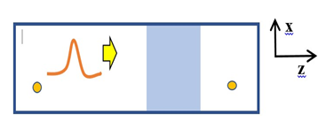
The geometry of this study was illustrated in Figure 1.We set the Gaussian pulse as a source which was drawn by red curve. This pulse propagated in the $\hat{z}$ direction. The blue rectangle was a dielectric barrier. Here, the two orange points were reflectance and transmittance points of measurement.

The simulation of electromagnetic waves using FDTD begin from the formulation of Ampere law : $\nabla \times \vec{H}\mathrm{=\epsilon }\frac{d\vec{E}}{\mathrm{dt}}$ and Faraday law: $\nabla \times \vec{E}\mathrm{=-\mu }\frac{d\vec{H}}{\mathrm{dt}}$ . Since we focused in only one dimension problems (for example: the propagation was in the z dimension), then two others dimension (the x and y dimensions) were not varied. It mean that the derivative with respect to x and y dimensions could be excluded from curl operation in Maxwell’s equations. Hence, the Ampere and Faraday laws in one dimension can be written as:

According to Ref.[1], the Maxwell equations in Eq.(1a) and (1b) could be brought to the spatial and temporal discretization as:

Here, n was used to discretize time while i was to discretize space. In every time step, the basic code for the electric and magnetic fields for the spatial discretization, then can be written as

Using Yee’s algorithm, Eq.(3) was derived from Eq.(2). Here, k represented the position of the fields in spatial discretization.

In our simulation, we implemented Gaussian pulse by adding the Gaussian fields at the certain position. However, we also required to have the propagation of the pulse in only one direction. It can be achieved by employing total fields/ scattering fields (tf/sf) method. Then, we had to add the fields such as:

where $k_{\mathrm{src}}$ represented the location of the source pulse, $H_{\mathrm{src}}$ was magnetic field source and T symbolised temporal grid. For the magnetic component, the form is relatively similar. We had to change $E_y\to H_x$ , $H_{\mathrm{src}}\to E_{\mathrm{src}}$ and $k_{\mathrm{src}}\to k_{\mathrm{src}}\mathrm{-1.}$ The simulation would be more realsitic, if the pulses were completely absorbed at the numerical boundary. Since, in this study, we focus in one dimension only, we used Dirichlet boundary condition at the numerical boundary. This simple method required that both electric and magnetic pulse were zero at the numerical boundary.

Results and Discussion

Firstly, we wanted to verified the results of the electromagnetic simulation. The results for the

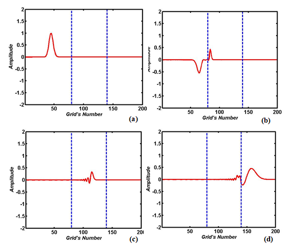
simulation of electromagnetic propagation were presented in Figure. 2. In that picture, the dotted blue lines represented the edge of dielectric barrier.

In our simulation, we set the medium inside numerical region was vacuum. From Figure 2, we took the propagation into four snapshoots. At time grid 150 ns (Fig.2a), the Gaussian pulse was generated and started to propagate at only in one direction: the z direction. When the propagation reached the dielectric object (at time grid 250 ns), the incoming pulse broke up into two parts, the transmitted waves and reflected waves. Later, at time grid 450 ns (see Fig.2c, the reflected waves were absorbed when they arrived at the numerical boundary. However, the transmitted waves continue to propagate inside the dielectric barrier. In Fig.2d, we noticed that the amplitude and phase of transmitted waves increase when they reached the end of dielectric barrier and propagated to vacuum. It happened since the permittivity of dielectric barrier was higher then the permittivity of vacuum. The transmitted pulse was also absorbed when it reached the numerical boundary.

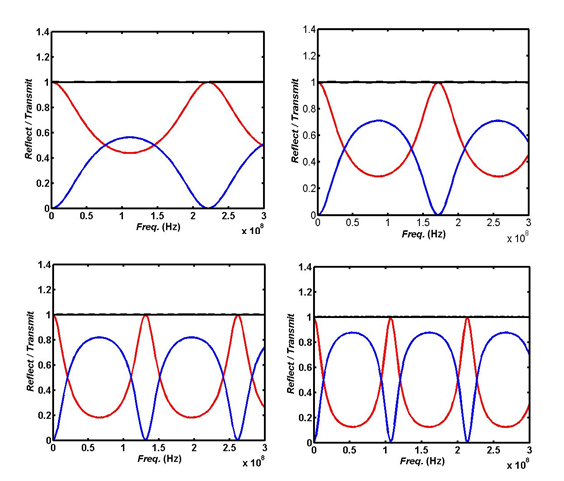
The results of transmittance and reflectance’s calculation was presented in figure 3. The solid red lines were represented transmittance (T), while the blue lines were reflectance (R). The addition of reflectance and transmittance, $\mathrm{R+T=1}$ , was illustrated as solid black lines. Here, from figure 3a to 3d, we varied the dielectric barrier by using dielectric materials such as: Mica ( ${\epsilon }_r\mathrm{=7),}$ Silicon (( ${\epsilon }_r\mathrm{=12)}$ , Acetone (( ${\epsilon }_r\mathrm{=20)}$ and Nitrobenzene (( ${\epsilon }_r\mathrm{=30).}$

It could be noticed from figure 3, that the average and the peak response of transmittance decreased when the permittivity was increased. As it was expected, the higher permittivity mean the denser the barrier, then the abbility for electromagnetic waves to propagate through barrier became decrease. For reflectance, it behaved in opposite way, the average and the peak response of reflectance increased when the permittivity of the barrier was getting bigger. These properties was also agree with the well known theory in optics. It was also seen that the number of the peak response for both transmittance and reflectance increased as the dielectric barrier with low permittivity was changed to the dielectric with high permittivity. In our argument, the permittivity was related to the number of phonon of a dielectric. Hence, it associated to the number of interaction between electromagnetic waves and phonon. As a result, the number of peak response was also connected to it.

Conclusion

The transmittance and reflectance was significantly affected by the permittivity of the object. The transmitance was small while the reflectance was high as the permittivity of the object was high. The permittivity also affected the number of peak response in both transmittance and reflectance. As the permittivity of the object was high, the number of the peak response was also high.

Acknowledgment

We highly acknowledge Physics Department, Faculty of Sciences and Mathematics, Diponegoro University for the support of this work .

References

- Yee, K. S., “Numerical Solution of Initial Boundary Value Problems Involving Maxwell’s Equations in Isotropic media”, IEEE Trans. Antennas Propagat.14, 302-307, 1966. . DOI ↗ Google Scholar ↗
- Mirza, A. F., Abdussalan, R., Asif, R., Darma, Y. A. S., Abussita, M. M., Elmegri, F., Abd-Alhamed, R. A., Noras, J. M.,\and Qahwaji, R.,” Breast Cancer Detection using 1D, 2D and 3D FDTD Numerical Methods”., 2015 IEEE International Conference on Computer and Information Technology; Ubiquitous Computing and Communications; Dependable, Autonomic and Secure Computing; Pervasive Intelligence and Computing, Liverpool, UK, 2015, pp. 1042-1045.. DOI ↗ Google Scholar ↗
- 3 Zulfa, V. Z., Farahdina, U., Firdhaus, M., Azis, I., Nasori, N., Darsono, D. and Rubiyanto, A.,” FDTD Simulation of Magnetic Field Distribution in Normal and Blood Cancer for Treatment”, J. Phys: Conf. Ser.1951 12061, 2021 DOI ↗ Google Scholar ↗
- Zheng, Z., Yiyang, L. and Jianjun, W., “Recent advances in surface enhanced Raman spectroscopy (SERS): finite difference time domain (FDTD) method for SERS and sensing applications”, Trends in Analytical Chemistry 75 162-173, 2016 (doi: DOI ↗ Google Scholar ↗
- Piltyay, S., Bulashenko, A., Herhil, Y. and Bulashenko, O., “FDTD and FEM Simulation of Microwave Waveguide Polarizers “, 2020 IEEE International Conference on Advanced Trends in Information Theory, Kyiv, Ukraine, 2020, pp. 357-363, . DOI ↗ Google Scholar ↗
- Giannakis, I., Giannopoulos, A. and Warren, C., “A Realistic FDTD Numerical Modeling Framework of Ground Penetrating Radar for Landmine Detection”, IEEE Journal of Selected Topics in Applied Earth Observations and Remote Sensing 9, 37-50, 2016, . DOI ↗ Google Scholar ↗
- Gao. S., , Li, W. L. and Sambell.A., , “FDTD Analysis of Dual-Frequency Microstrip Patch Antenna”, Progress In Electromagnetic Research 54, 155-178, 2005. . DOI ↗ Google Scholar ↗