Abstract
The high-speed railways require more viaducts/bridges than a conventional railway. The dynamic analysis of viaduct-like structures under the passage of high-speed trains is im-portant due to comfortable riding, the safety of via-ducts/bridges, safe running, risk of derailment, etc. In this study, it is investigated which mode shapes are dominant on the dynamic response of a viaduct subjected to a high-speed train. The viaduct is modelled as a multi-bay frame and the train is modelled as a four-axle two-bogie multi-body system with 10 degrees of freedom. The finite ele-ment method, based on the Bernoulli-Euler beam theory, is used to discretize the equations of motion. The Wilson-theta time integration scheme is employed to determine the dynamic response of the structure. To determine which modes dominate the dynamic response, three-dimensional (3D) relationship of frequency-velocity-amplitude graphs are plotted. It has been determined that the resonant re-sponse has been encountered at first and second modes of 1 and 2-bay frames and first, second and third modes of 3-bay frames.
Keywords
viaduct mode shape the finite element method the Wil-son-theta method moving train
1. Introduction
Dynamic responses of structures, such as bridges, and viaducts under the action of trainloads have seen considerable interest in the field of civil engineering. With the development of high-speed trains, the dynamic analysis of railway bridges has become important.
Viaducts are used mainly to connect two points of the terrain which have a similar height to carry mostly rail and road traffic. Su et al. [1] studied the dynamic responses of a viaduct subject to a high-speed train. 3D dynamic analysis models for the train-bridge system were developed. The train was idealized as a four-axle two-bogie with 27 degrees of freedom (DOF) dynamic system. The dynamic responses have been investigated using field measurement and numerical simulations. Track irregularities have been considered in this study. The authors [2][8] have modelled for both the vehicle and the structure as 3D dynamic systems in their papers.
Dynamic analysis of a structure subjected to a moving vehicle requires an accurate model. Lou et al. [9] have presented a modal coordinate formulation for analyzing the dynamic interaction between a simply supported bridge and a moving train. The train is modelled as a two-stage suspension vehicle with 10 DOF. Based on the Euler-Bernoulli beam theory, the bridge is modelled as a uniform simply supported beam. Rayleigh damping is assumed for the bridge. Ju et al. [10] examined train induced vibrations using field measurements and theoretical solutions. The study in the paper was shown that when the train moves at both subsonic and supersonic train speeds train-induced ground vibration at the trainload dominant frequencies are considerably large. In the literature, the dynamic behavior of structures subjected to a four-axle two-bogie train with 10 unconstrained degrees of freedom is investigated by authors [11][16]. Other train models, such as those 2-axle 6 DOF [17], 4 DOF [18, 19]; moving suspension mass model [20].
Today, the use of high-speed trains as a means of transportation is becoming more and more common. Due to the high speeds of these trains, the high-speed train lines should be approximately flat. As a result of this requirement, viaducts are used extensively on high-speed train lines. In some lines, the ratio of viaduct/bridge length to line length exceeds 80%, depending on the geographical conditions of the country [2].
Dynamic analysis of bridges under the influence of moving vehicles has been extensively studied in the literature. In these studies, the bridge is modelled as a simply supported beam [9, 13, 14]. For this bridge model, it has been shown that considering only the first mode of the structure gives rather accurate solutions for the dynamic response of both the bridge and the vehicle [21]. Due to a load in the vertical direction will be applied to the structure by the vehicle, a vibration mode with dominant vertical displacements will be excited. Since the viaduct structures are composed of beams and columns, and also because the dominant vibration modes in the axial direction have a lower frequency than the dominant vibration modes in the vertical direction, more vibration modes need to be considered. In the existing literature, there are few publications in which the viaduct is modelled as a frame structure and applied to vehicle-structure interaction dynamics problems. Demirtaş et al. [22] investigated the dynamic response and resonance characteristics of cracked multi-bay frame structures subjected to moving oscillatory loads, highlighting the influence of crack location on the dominant vibration modes. In addition, to the best of the author's knowledge, there is no study examining the effect of mode shapes on in-plane vibrations of viaduct-like structures. In this study, which vibration modes are dominant in the resonance vibrations of the structure were investigated in detail.
The resonant response of the train-bridge system is of particular interest due to the structural safety of the bridge, risk of derailment and deterioration of passenger comfort. Resonance occurs if one of the dominant frequencies of the trainload equals a multiple of one of the natural frequencies of the structure. The lower natural frequencies of the structures used in high-speed train lines mean that the structure can resonate at a smaller speed value. In this study, the dominating modes of the dynamic response of the viaduct are investigated by using the finite element method. Three-dimensional frequency-speed-amplitude graphs are plotted for this purpose. It was determined whether the peaks in this graph force the structure under resonance conditions.
Frame structures, for instance, gantry cranes, bridges, viaducts, etc. having the combination of beams and columns, subjected to moving trains are often encountered in engineering applications. In this study, the viaduct is thought to be modelled as a multi-bay frame. The multi-bay frame, based on Bernoulli-Euler beam theory, has the boundary conditions of zero horizontal and vertical displacements and zero rotations at the bases of columns. Also, the train is idealized as a four-axle two-bogie multi-body system with 10 degrees of freedom.
2. Theory
2.1 System description
The problem to be dealt with in the present study is a multi-bay frame subjected to moving train, shown in Fig. 1. Bernoulli-Euler beams forming the frame have the beam (column) length L, the elastic modulus Ebe, the area moment of inertia Ibe, and the mass per unit length mbe. The points p1 and p2 are corresponding to midpoint of the column and top beam, respectively.
The vehicle model representing a train consists of primary and secondary suspension systems having stiffness kp and ks; damping cp and cs. The mb, mw and mv are the mass of a bogie, the mass of a wheelset and mass of a vehicle body, respectively. Jb and Jv are the corresponding mass moments of inertia of a bogie and vehicle body. Ld is the longitudinal distance between the center of gravity of bogie and the nearest side of vehicle body. d1 (d2) is the horizontal distance between the center of gravity of the vehicle body and of rear (front) bogie. Lb is the half of bogie axle base. G is the center of gravity of the vehicle body [25].
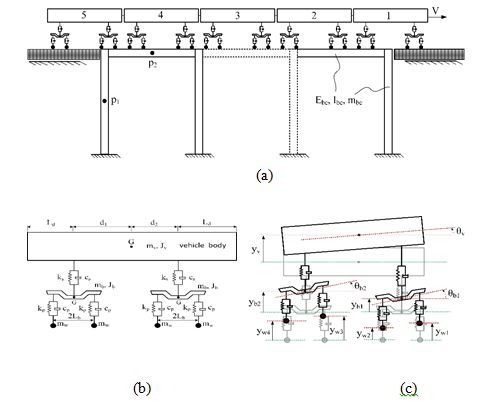
As seen Fig. 1(c), ywi(t) (i=1,2,3,4) denote the vertical displacement of the ith wheelset. yb1 and yb2 are the vertical displacements of bogies and yv is vertical displacement of the vehicle body. Also, θbi(i=1,2) and θv are rotations of bogies and vehicle body. The vehicle has ten unconstrained degrees of freedom. It is assumed that the upward vertical displacements are taken as positive and that they are measured from the respective static equilibrium positions.
2.2 Vehicle-structure interaction dynamics
In this study, a four-axle vehicle travelling at a uniform speed V on a multi-storey frame is investigated, shown in Fig. 2. xi(t) (i=1,2,3,4) are the contact points between the frame and ith axle measured from the left end of the top beam. It is assumed that four wheelsets and frame are in contact with elements ei (i=1,2,3,4) at a time t. q1ei and q4ei (i=1,2,3,4) denote the vertical displacements at nodes of element ei.
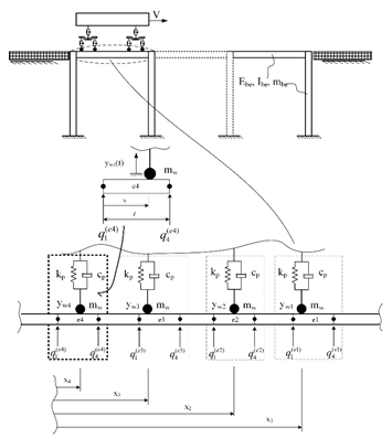
The equation of motion of the frame and vehicle are derived from the following generalized Lagrangian equation:
Here, q ̇ and q are respective generalized velocities and displacements of the whole system.
The potential energy of the vehicle consists of primary and secondary suspension systems. The kinetic energy of the vehicle is formed by the mass of the bogies, the mass of the wheelsets, and the mass of the vehicle's body. The dissipation function term comes from primary and secondary suspension systems. Those are related to displacements and velocities in the vertical directions of the vehicle's corresponding components. The kinetic energy and elastic strain energy of the frame are comprising both the vertical and the horizontal movement of the frame. The kinetic energy, potential energy and dissipation function of the integrated system can then be written as
where Mf and Kf are the mass and stiffness matrices of the frame [23]. qf and q ̇ f are the vectors of nodal displacement and velocity of the frame, respectively.
The total number of degrees of freedom of the vehicle is ten. It is assumed that the wheels always keep in contact with the structure. This indicates that the structure and wheelsets do not move independently from each other. Therefore, the vertical displacement/velocity of each wheelset is equal to the vertical displacement/velocity of the point where it contacts the frame [25]:
where the derivative of a function f(x) with respect to x is denoted by f(x),x, ξ = x/l (see Fig. 3) and Ni (i=1,2,...,6) are interpolation functions:
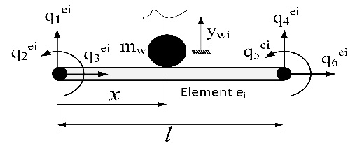
Nodal degrees of freedom of the element ei is shown in Fig. 3 and the nodal displacement vector is as follows:
and displacement vector of vehicle is following:
After some algebraic manipulations, the following equations of motion for the system can be obtained
where the subscripts v and f represent the vehicle and the frame, respectively. The index vf (or fv) in matrices is the result of the interaction between the structure and the vehicle. Mfv, Cfv and Kfv are the NxN matrices and C ̅ vf and K ̅ vf are Nx6 matrices. The the non-zero columns of these matrices are given in appendix.
When the vehicle runs on the structure, matrices with double subscript and the vector of f are always changing. As a consequence of this, Eq. 10 becomes a second-order differential equation with variable coefficients. Those time-variable coefficients should be updated every time interval before numerical integration process apply. Eq. 10 can then be solved by using the Wilson-theta time integration scheme with θ=1.4 [24,2].
Validation model
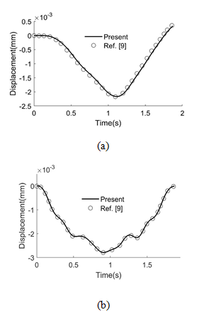
A simply supported beam subjected to a single vehicle is considered. The example model has been studied by Lou et al. [9]. Fig. 4 show good agreement between present model and model in Ref. [9].
3. Determination of the dominant mode shapes of the multi-bay frame
The present work based on the theory presented above is applied to the study given below: (1) the first few natural frequencies are calculated and their mode shapes are plotted. (2) The 3D relationship of velocity-frequency-amplitude graphs is established. The values of frequency and velocity at the peak points in 3D graphs are extracted. The critical speeds can then be identified when bridge deflection reaches the maximum value. (3) The mode shapes that affect the resonance response of the structure are obtained by plotting the time history of the points taken.
All the parameters which are used in subsequent computations have been given in Table 1. The values of physical properties are taken from [9].
| Description | Notation | Value |
| Vehicle | ||
| Mass of the vehicle body | mv | 4.175x10³ kg |
| Mass of a wheelset | mw | 1.78x10³ kg |
| Mass moment of inertia of vehicle body | Jv | 2.08x10⁶ kg.m2 |
| Horizontal distance between the center of gravity of car body and of rear bogie | d1 | 8.75 m |
| Horizontal distance between the center of gravity of car body and of front bogie | d2 | 8.75 m |
| Longitudinal distance between the center of gravity of bogie and nearest side of vehicle body | Ld | 3 m |
| Stiffness of primary suspension system | kp | 1.18x10⁶ N/m |
| Damping of primary suspension system | cp | 3.92x10⁴ N.s/m |
| Stiffness of secondary suspension system | ks | 5.3x10⁵ N/m |
| Damping of secondary suspension system | cs | 9.02x10⁴ N.s/m |
| Mass bogie | mb | 3.04x10³ kg |
| Mass moment of inertia of a bogie | Jb | 3.93x10³ kg.m2 |
| Half of bogie axle base | Lb | 1.25 m |
| Multi-bay frame | ||
| Beam/column length of frame | L | 25 m |
| Mass moment of inertia | Ibe | 2.9 m4 |
| Mass per unit length | mbe | 1.2x10⁴ kg/m |
| Young’s modulus | Ebe | 109 Pa |
3.1 Modal analysis of the multi-bay frame
The first few natural frequencies are determined using both ANSYS and the developed MATLAB programs (present work). The beams and columns are modelled using the BEAM54 element. ANSYS BEAM54 is used because it has the same nodal degrees of freedom as the model developed by the present work. Element size is taken as 5 m to generate the same finite element mesh those the developed model. Table 2 shows the natural frequencies of i-bay frame (i=1, 2, 3).
| 1-bay | 2-bay | 3-bay | ||||
| f(Hz) | Present work | ANSYS | Present work | ANSYS | Present work | ANSYS |
| f1 | 0.4714 | 0.47135 | 0.4370 | 0.4370 | 0.4256 | 0.4255 |
| f2 | 1.8477 | 1.8442 | 1.7933 | 1.7898 | 1.7709 | 1.7675 |
| f3 | 3.0356 | 3.0267 | 2.2309 | 2.2265 | 2.0219 | 2.0179 |
| f4 | 3.2412 | 3.2343 | 3.0555 | 3.0469 | 2.4501 | 2.4452 |
| f5 | 3.0644 | 3.0559 | ||||
| f6 | 3.1410 | 3.1352 | ||||
| f7 | 3.2408 | 3.2340 |
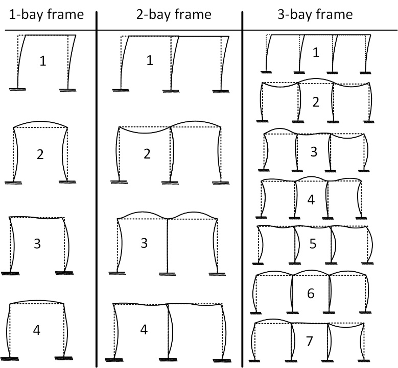
The mode shapes corresponding to natural frequencies given in Table 2 are plotted. The first modes of the structures shown in Fig. 5 are related to the first bending modes of the columns forming the frame. The vertical displacements of the top beam are negligible in these modes. Due to train travelled on the top beam, it can be expected that mode shapes in which vertical displacements of the top beam are effective are important on resonance response. Therefore, the 2nd and 4th modes of the 1-bay frame; the 2nd and 3rd modes of the 2-bay frame and the 2nd, 3rd, 4th, 6th and 7th modes of the 3-bay frame may be effective in resonance response of the structure.
3.2 Velocity-frequency-amplitude graphs
3D relationship of velocity-frequency-amplitude graphs was plotted with respect to horizontal displacements of the point p1 and vertical displacements of the point p2 (see Fig. 1 (a)). The displacement-time history curves of the i-bay frame (i=1, 2, 3) was first determined at each velocity (V=1, 2, ...,100). Then, frequency responses were obtained by applying the Fourier transform to free vibrations. It should be noted that the number of vehicles was taken as 5 when plotting 3D graphics. However, to better visualize resonance, the number of vehicles in the displacement-time history curves was selected as 10.
1-bay frame
Fig. 6 shows the 3D views of the velocity-frequency-amplitude plot. There exists 3 peaks in Fig. 6 (a). The velocities corresponding to the peaks of amplitude may be viewed as the critical velocities at which the resonance vibration may occur. Those velocities and frequencies can be read as f1 =0.47 Hz, V=11 m/s; f2 =1.847 Hz, V=45 m/s and f3 =3.04 Hz, V=73 m/s. From Fig. 6 (b), two peak amplitudes can be extracted as f2=1.847 Hz, V=45 m/s and f4=3.24 Hz, V=77 m/s.
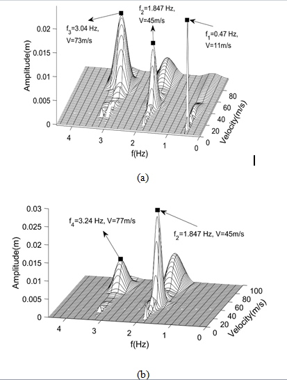
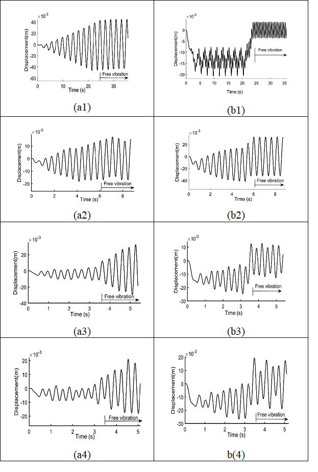
Fig. 7 shows displacement-time history curves for velocities of 11, 45, 73 and 77 m/s. Fig. 7 (a1) is related to resonance behavior in horizontal direction. As the vehicle interacts with the structure, the vibration amplitudes of the structure have increased over time. After the vehicle passes over the frame, it is clear that free vibrations with constant amplitude have occurred. Fig. 7 (b1) shows the vertical displacements of the point p2. It can be stated that the displacements in the vertical direction are small compared to the displacements in the horizontal direction. As the 1st mode shape of the structure (see Fig. 5) is examined, it is determined that this displacement pattern is corresponding to the 1st mode shape of the 1-bay frame. The velocity V=11 m/s has excited the first mode of vibrations.
The resonant responses both in the horizontal and vertical directions are encountered when the speed of the train has a velocity of V=45 m/s. This critical speed excites the 1-bay frame in 2nd mode of vibrations. The amplitude of vibration in the vertical direction takes place at the maximum value when compared with Figs. 7 (b1), (b3) and (b4). As seen in Figs. 7 (a3), (b3), (a4) and (b4), the resonance behavior in connection with 3rd and 4th modes cannot appear within these velocity range.
2-bay frame
The 3D relationship of velocity-frequency-amplitude graphs are given in Fig. 8. The four possible peaks which may cause resonance vibrations in the horizontal direction at point p1 are shown in Fig. 8 (a). The velocity and frequency values corresponding to these peak amplitudes are as follows: f1 = 0.437 Hz, V = 11 m/s; f2 = 1.79 Hz, V = 42 m/s; f3 = 2.23 Hz, V = 57 m/s and f4 = 3.05 Hz, V = 74 m/s. It is clear that the largest amplitude occurs when f1 = 0.437 Hz, V = 11 m/s. In both Figs. 8 (a) and 8 (b), peaks occurs at f2 = 1.79 Hz, V = 42 m/s and f3 = 2.23 Hz, V = 57 m/s. As observed in the previous case, it is seen that the vibrations with the largest amplitude occur at the velocity of the vehicle at low speed, which is related to the first mode of the frame.
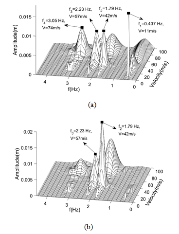
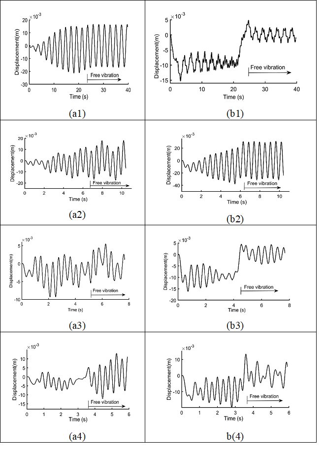
Fig. 9 (a1) depicts the resonant response in horizontal direction. It is also obvious that the vertical displacements of the point p2 are small at the same velocity value. These are the displacement characteristics of the 1st mode. In Figs. 9 (a2) and (b2), the resonance response has encountered both in the horizontal vibrations of the point p1 and the vertical vibrations of the point p2. Therefore, the 2nd mode of the frame is also effective in causing a resonance response. From Figs. 9 (a3), (b3), (a4) and (b4), the resonant response does not exist for those critical velocities.
3-bay frame
With the increase in the number of bays of the frame, the natural frequencies have become close to each other (see Table 2). As can be seen in in Fig. 10(a), there are five amplitude peaks. The critical velocity and its corresponding frequency values in Fig. 10 (a) are: f1 = 0.426 Hz, V = 11 m/s; f2 = 1.77 Hz, V = 39 m/s; f3 = 2.02 Hz, V = 49 m/s; f4 = 2.45 Hz, V = 55 m/s and f7 = 3.24 Hz, V = 77 m/s. Three of these peak points are also seen in Fig. 10 (b): (f2 = 1.77 Hz, V = 39 m/s), (f3 = 2.02 Hz, V = 49 m/s) and (f7 = 3.24 Hz, V = 77 m/s).
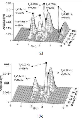
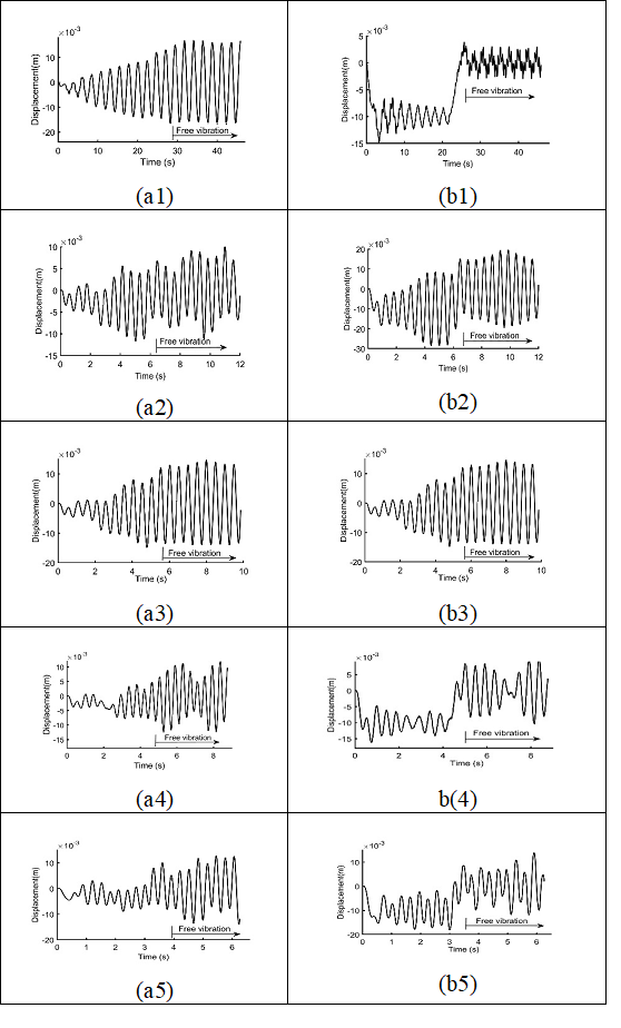
Fig. 11 illustrates the displacement-time curves for the above-mentioned velocities. One observation here is that as in 1 and 2-bay frames, the resonance vibrations are encountered at the critical velocity of V=11 m/s. In addition, the critical speeds for the resonance response to occur are found at 39 m/s and 49 m/s. In those velocities, 2nd and 3rd modes have been excited. Another observation is that unlike the 1 and 2 bay frames, the resonance effect also takes place in the 3rd mode of the 3-bay frame (Figs. 11 (a3)-(b3)). It is evident that the resonant behavior is not observed at the critical speeds of V=55 m/s, 77 m/s and corresponding mode 4th and mode 5th.
The first natural frequencies of the i-bay (i = 1,2,3) frame are very close to each other. Note that the critical speed values that excite this mode are the same which is 11 m/s, due to the graphs being plotted in increments of 1 m/s. It is also pointed out that the maximum value of the amplitudes decreased as the number of bays of the frame increased, as seen in Figs. 6, 8 and 10.
4. Conclusions
The study dealt with in this paper investigates the effect of mode shapes on the dynamic response of the viaduct, based on the Bernoulli-Euler beam theory, subjected to a train moving at velocity v. The viaduct is modelled as a multi-bay frame by using the finite element method. The train is modelled as a four-axle two-bogie multi-body system with 10 DOF. The equations of motion of the integrated vehicle-structure system are obtained by using generalized Lagrange's equations. To integrate the equations of motion, the Wilson-theta method is employed. The amplitude spectrum is determined by applying the Fourier transform on the free-response part of the displacement-time history. The 3D relationship of velocity-frequency-amplitude graphs at points p1 and p2 are then plotted. The dominant modes related to resonance response are determined. The resonance phenomenon has occurred in the 1st mode of the 1, 2 and 3-bay frames, the 2nd mode of the 1, 2 and 3-bay frames and the 3rd modes of the 3-bay frame. However, resonance vibrations are not encountered in the 3rd and 4th modes of the 1 and 2-bay frames and the 4th and 7th modes of the 3-bay frame, except for the 1st mode of the i-bay frame (i=1, 2, 3), where vertical displacements are negligible. The amplitude of the resonance vibrations is decreased as the number of bays of the frame is increased.
In Eq. (10), the following abbreviations have been introduced:
M fv i < q 1 e i >= [ 0 … m w N 1 2 0 0 m w N 1 N 4 0 0 … 0 ] T M fv i < q 4 e i >= [ 0 … m w N 1 N 4 0 0 m w N 4 2 0 0 … 0 ] T (A1)
C fv i < q 1 e i >=[ 0 ⋮ ⋮ 2V m w N 1 N 1,x + c p N 1 2 0 0 2V m w N 1,x N 4 + c p N 1 N 4 0 0 ⋮ ⋮ 0 ], C fv i < q 4 e i >=[ 0 ⋮ ⋮ 2V m w N 1 N 4,x + c p N 1 N 4 0 0 2V m w N 4 N 4,x + c p N 4 2 0 0 ⋮ ⋮ 0 ] (A2)
K fv i < q 1 e i >=[ 0 ⋮ ⋮ m w V 2 N 1 N 1,xx + c p V N 1 N 1,x + k p N 1 2 0 0 m w V 2 N 1 N 4,xx + c p V N 1 N 4,x + k p N 1 N 4 0 0 ⋮ ⋮ 0 ], K fv i < q 4 e i >=[ 0 ⋮ ⋮ m w V 2 N 1,xx N 4 + c p V N 1,x N 4 + k p N 1 N 4 0 0 m w V 2 N 4 N 4,xx + c p V N 4 N 4,x + k p N 4 2 0 0 ⋮ ⋮ 0 ] (A3)
where i=1, 2, 3, 4.
A ‾ fv =[ 0 0 0 0 0 0 0 - a p N 1 0 0 a p L b N 1 0 0 0 0 0 0 0 0 0 0 0 0 0 0 - a p N 4 0 0 a p L b N 4 0 ⋮ ⋮ ⋮ ⋮ ⋮ ⋮ 0 - a p N 1 0 0 - a p L b N 1 0 0 0 0 0 0 0 0 0 0 0 0 0 0 - a p N 4 0 0 - a p L b N 4 0 ⋮ ⋮ ⋮ ⋮ ⋮ ⋮ - a p N 1 0 0 a p L b N 1 0 0 0 0 0 0 0 0 0 0 0 0 0 0 - a p N 4 0 0 a p L b N 4 0 0 ⋮ ⋮ ⋮ ⋮ ⋮ ⋮ - a p N 1 0 0 - a p L b N 1 0 0 0 0 0 0 0 0 0 0 0 0 0 0 - a p N 4 0 0 - a p L b N 4 0 0 0 0 0 0 0 0 ] (A4)
M v =diag( m b , m b , m v , J b , J b , J v ) (A5)
A v =[ 2 a p + a s 0 - a s 0 0 - d 1 a s 0 2 a p + a s - a s 0 0 d 2 a s - a s - a s 2 a s 0 ( d 1 - d 2 ) a s 0 0 0 0 2 L b 2 a p 0 0 0 0 0 0 2 L b 2 a p 0 - d 1 a s d 2 a s ( d 1 - d 2 ) a s 0 0 ( d 1 2 + d 2 2 ) a s ] (A6)
f = [ 0 … f 1 e i 0 0 f 4 e i 0 0 … 0 ] T (A7)
where f 1 ei and f 4 ei represent the vehicle loads exerted by each wheelset on the contacting element i and those are determined as follows:
f 1 e i =-( m w + 1 2 m b + 1 2 m v d 2 d 1 + d 2 )g N 1 f 4 e i =-( m w + 1 2 m b + 1 2 m v d 1 d 1 + d 2 )g N 4 (A8)
where g is the acceleration due to gravity.
Notation A < q j ei > represents the jth column of the element ei in the matrix A. If A and a in matrices A ̅ vf and A v in Eqs. (A.4) and (A.6) are replaced by C and c (or K and k), matrices C ̅ vf and C v (or matrices K ̅ vf and K v ) can be determined.
Acknowledgements Not applicable.
Author contributions All the authors have equally contributed to the work.
Funding Not applicable
Data availability statement Not applicable
Declarations
Conflict of interest. The authors declare that they have no known competing financial interests or personal relationships that could have appeared to influence the work reported in this paper.
References
- Su D, Fujino Y, Nagayama T, Hernandez JY, Seki M. Vibration of reinforced concrete viaducts under high-speed train passage: Measurement and prediction including train-viaduct interaction. Bridge Struct. 2010;6(5):621-633. doi:. DOI ↗ Google Scholar ↗
- Guo WW, Xia H, De Roeck G, Liu K. Integral model for train-track-bridge interaction on the Sesia viaduct: Dynamic simulation and critical assessment. Comput Struct. 2012;112-113:205-216. doi:. DOI ↗ Google Scholar ↗
- Romero A, Solís M, Domínguez J, Galvín P. Soil-structure interaction in resonant railway bridges. Soil Dyn Earthq Eng. 2013;47:108-116. doi:. DOI ↗ Google Scholar ↗
- Xia CY, Lei JQ, Zhang N, Xia H, De Roeck G. Dynamic analysis of a coupled high-speed train and bridge system subjected to collision load. J Sound Vib. 2012;331(10):2334-2347. doi:. DOI ↗ Google Scholar ↗
- Majka M, Hartnett M. Effects of speed, load and damping on the dynamic response of railway bridges and vehicles. Comput Struct. 2008;86(6):556-572. doi:. DOI ↗ Google Scholar ↗
- Nokhbatolfoghahai A, Noorian MA, Haddadpour H. Dynamic response of tank trains to random track irregularities. Meccanica. 2018;53(10):2687-2703. doi:. DOI ↗ Google Scholar ↗
- Dimitrakopoulos EG, Zeng Q. A three-dimensional dynamic analysis scheme for the interaction between trains and curved railway bridges. Comput Struct. 2015;149:43-60. doi:. DOI ↗ Google Scholar ↗
- Lee YS, Kim SH. Structural analysis of 3D high-speed train-bridge interactions for simple train load models. Veh Syst Dyn. 2010;48(2):263-281. doi:. DOI ↗ Google Scholar ↗
- Lou P, Dai GL, Zeng QY. Modal coordinate formulation for a simply supported bridge subjected to a moving train modelled as two-stage suspension vehicles. Proc Inst Mech Eng Part C J Mech Eng Sci. 2005;219(10):1027-1040. doi:. DOI ↗ Google Scholar ↗
- Ju SH, Lin HT, Huang JY. Dominant frequencies of train-induced vibrations. J Sound Vib. 2009;319(1-2):247-259. doi:. DOI ↗ Google Scholar ↗
- Duan YF, Wang SM, Wang RZ, Wang CY, Shih JY, Yun CB. Vector form intrinsic finite-element analysis for train and bridge dynamic interaction. J Bridge Eng. 2018;23(1):04017117. doi:. DOI ↗ Google Scholar ↗
- Hubbell D, Gauvreau P. Frequency domain analysis of train-guideway interaction dynamics. J Struct Eng. 2018;144(8):04018099. doi:. DOI ↗ Google Scholar ↗
- Wu YS, Yang YB. Steady-state response and riding comfort of trains moving over a series of simply supported bridges. Eng Struct. 2003;25(2):251-265. doi:. DOI ↗ Google Scholar ↗
- Youcef K, Sabiha T, El Mostafa D, Ali D, Bachir M. Dynamic analysis of train-bridge system and riding comfort of trains with rail irregularities. J Mech Sci Technol. 2013;27(4):951-962. doi:. DOI ↗ Google Scholar ↗
- Biondi B, Muscolino G, Sofi A. A substructure approach for the dynamic analysis of train-track-bridge system. Comput Struct. 2005;83(28-30):2271-2281. doi:. DOI ↗ Google Scholar ↗
- Hirzinger B, Adam C, Salcher P, Oberguggenberger M. On the optimal strategy of stochastic-based reliability assessment of railway bridges for high-speed trains. Meccanica. 2019;54(9):1385-1402. doi:. DOI ↗ Google Scholar ↗
- Xiang T, Zhao R, Xu T. Reliability evaluation of vehicle-bridge dynamic interaction. J Struct Eng. 2007;133(8):1092-1099. doi:). DOI ↗ Google Scholar ↗
- Yang YB, Chang CH, Yau JD. An element for analysing vehicle-bridge systems considering vehicle pitching effect. Int J Numer Methods Eng. 1999;46:1031-1047. <1031::aid-nme738>3.3.co;2-m DOI ↗ Google Scholar ↗
- Stancioiu D, Ouyang H, Mottershead JE. Vibration of a continuous beam with multiple elastic supports excited by a moving two-axle system with separation. Meccanica. 2009;44(3):293-303. doi:. DOI ↗ Google Scholar ↗
- Lin CC, Wang JF, Chen BL. Train-induced vibration control of high-speed railway bridges equipped with multiple tuned mass dampers. J Bridge Eng. 2005;10(4):398-414. doi:). DOI ↗ Google Scholar ↗
- Yang YB, Lin CW. Vehicle-bridge interaction dynamics and potential applications. J Sound Vib. 2005;284:205-226. doi:. DOI ↗ Google Scholar ↗
- Demirtaş S, Ozturk H, Kiral Z. Vibration characteristics of a cracked multi-bay frame with moving oscillatory loads. Bridge Struct. 2025;21(4):180-197. doi:. DOI ↗ Google Scholar ↗
- Demirtas S, Ozturk H, Sabuncu M. Dynamic response of multi-bay frames subjected to successive moving forces. Int J Struct Stab Dyn. 2019;19(4):1950042. doi:. DOI ↗ Google Scholar ↗
- Bathe KJ. Finite Element Procedures. 2nd ed. Upper Saddle River (NJ): Prentice Hall; 1996. DOI ↗ Google Scholar ↗
- Demirtaş S. Vibration analysis of complex structures subjected to moving loads [doctoral dissertation]. İzmir (Türkiye): Dokuz Eylul University; 2020. DOI ↗ Google Scholar ↗