Abstract
Public co-location datasets are increasingly used to develop and benchmark machine-learning calibrations for low-cost air quality sensors, yet they are rarely audited before use. We audited an openly licensed dataset from Valencia, Spain, in which two ZPHS01B sensor nodes were co-located with a regulatory station for 237 days, and measured how its defects change calibration results. The audit found reference ozone values up to 97,336 µg m⁻³, several of them exact squares or cubes of plausible concentrations; constant sentinel-like negative values in the reference CO series; a humidity column that duplicates PM₁; hourly files that do not match the 10-minute files; low-cost CO and NO₂ channels that were effectively dead; stuck ozone output in up to 79 % of a node’s monthly records; and two “independent” nodes whose records are identical for the first eight weeks. The evaluation design mattered most. A gradient-boosting model given the date as a feature scored R² = 0.83 on a random 90/10 split but R² = −0.22 on the final tenth of the record. Leaving quality control out or keeping stuck segments shifted results further. We propose a short audit checklist for publishers and users of co-location data.
Keywords
low-cost sensors data quality co-location calibration data leakage machine learning reproducibility air quality
Introduction
The low-cost sensor literature has a quiet dependency problem. Calibration methods are developed, compared and published on a small number of co-location datasets, in which sensors sit beside a reference analyser for weeks or months. Reviews of the field cite dozens of calibration algorithms, from linear regression to deep learning (Concas et al., 2021; Liang, 2021; Kang et al., 2022). They include random forests (Zimmerman et al., 2018), general calibration models for whole networks (Malings et al., 2019; deSouza et al., 2022), open-source field calibration pipelines (Schmitz et al., 2021) and online learners built to cope with concept drift (Gama et al., 2014; Bagkis et al., 2022). Much of that progress is measured on data that few people have examined line by line. Recent open releases have widened access considerably. SensEURCity, for example, provides raw sensor and reference data from three European cities (Van Poppel et al., 2023). The same openness makes it easy to download a dataset, fit a model and report a number without asking whether the data can support the claim.
Machine learning has learned this lesson the hard way. Sambasivan et al. (2021) described “data cascades”, in which small upstream data problems compound into failures far downstream, often unnoticed. Kapoor and Narayanan (2023) traced a reproducibility crisis in machine-learning-based science largely to leakage between training and test data. Gebru et al. (2021) proposed datasheets so that every dataset arrives with an account of how it was collected, processed and should be used, and Whang et al. (2023) argued for treating data quality as a first-class part of model development. In atmospheric measurement, Diez et al. (2022) made a similar case: error characteristics determine whether data are fit for a given purpose, and that has to be established, not assumed.
Low-cost sensor data are especially exposed to these risks. Sensors age, saturate and get stuck (Li et al., 2021; deSouza et al., 2023), and best-practice guidance for calibration stresses careful screening of both sensor and reference data before any model is fitted (Giordano et al., 2021; Okorn and Iraci, 2024). Reference data are not error-free either; they come with their own invalid values, maintenance gaps and processing artefacts. Calibration studies are also unusually vulnerable to temporal leakage. Pollutant concentrations and weather are strongly autocorrelated, so a model tested on hours interleaved with its training hours can appear accurate while having learned little that transfers to the future (Nowack et al., 2021; Abu-Hani et al., 2024).
This paper audits one recent public dataset in detail and measures what its problems do to calibration results. The dataset, released under an open licence by researchers at the Universitat de València, contains about eight months of co-located data from two ZPHS01B multi-sensor nodes and a regulatory station in Valencia, Spain (Montalbán Faet et al., 2025). It supports a published study of ozone calibration with machine learning (Montalbán-Faet et al., 2025). We chose it because it is recent, well described on its landing page and typical of what a researcher, or a student starting a thesis, might pick up today. The documentation even warns users about some of the problems. Our aim is not to criticise the data creators, who made their data open when most groups do not, but to show how much can sit below the surface of a typical release and how far it moves the results.
The study has three objectives: (i) to apply a systematic set of checks covering completeness, plausibility, consistency, sensor health and provenance; (ii) to quantify how the defects found, and the evaluation design, change the apparent skill of standard calibration models; and (iii) to turn the lessons into a short checklist for those who publish and those who reuse co-location data. The checklist is meant to be useful well beyond Valencia. It is particularly relevant where networks are being built quickly with limited reference infrastructure, as in Nigeria and across sub-Saharan Africa (Awokola et al., 2022; Raheja et al., 2023).
Data and methods
The dataset
The release (Montalbán Faet et al., 2025) contains nine CSV files: reference data from the Molí del Sol station (gva_*.csv) and data from two low-cost nodes (n1_*.csv, n2_*.csv), each at 10-, 30- and 60-minute resolution. The reference files report SO₂, CO, O₃, NO, NO₂, NOₓ, PM₁, PM₂.₅, PM₁₀, sound level and several auxiliary variables. The node files report temperature, relative humidity (RH), PM₁, PM₂.₅, PM₁₀, VOC, formaldehyde, CO₂, CO, O₃ and NO₂ from a ZPHS01B module. Ozone is identified as the primary reference variable and the primary variable to calibrate. The landing page notes outliers and negative values in the reference data, missing values in the aggregated files, an erroneous humidity column, a frequently saturated NO₂ sensor and humidity readings above 100 %. Our audit confirms each of these and adds several that are not mentioned.
Audit checks
We grouped the checks into five families (Table 1). Each was applied to every variable where it made sense, mainly at 10-minute resolution.
| Family | Check | Rule used |
|---|---|---|
| Completeness and timing | Regular time grid; gaps | Count of steps longer than 10 min |
| Cross-resolution consistency | Hourly mean of 10-min file versus 60-min file, Eq. (6) | |
| Plausibility | Physical range | Eq. (1), limits per pollutant |
| Contaminated episodes | Eq. (2) | |
| Isolated spikes | Hampel filter, Eq. (3) | |
| Consistency | Duplicate or mislabelled columns | Exact equality between columns |
| Duplicated instrument streams | Eq. (5) across the two nodes | |
| Sensor health | Stuck or stale output | Flat-run length, Eq. (4) |
| Saturation and dead channels | Share of records at a single value or ceiling | |
| Provenance | Documentation versus data | Each documented caveat checked against the files |
For a variable c with value v c , t at time t , the range flag is
where 1 ⋅ is the indicator function and L c , U c are lower and upper plausibility limits. We used L c = 0 for every pollutant and upper limits well above anything expected at an urban background site: 300 µg m⁻³ for O₃, 400 µg m⁻³ for NO₂, 1000 µg m⁻³ for NO, 1500 µg m⁻³ for NOₓ, 350 µg m⁻³ for SO₂, 10 ppm for CO and 200, 500 and 150 µg m⁻³ for PM₂.₅, PM₁₀ and PM₁ respectively.
Isolated range violations are easy to remove. Clustered violations suggest an episode in which the instrument or the processing chain was misbehaving, and values that happen to fall inside the range during such an episode are also suspect. We therefore flagged a whole day d for variable c when
Remaining isolated spikes were detected with a Hampel filter. A value is flagged when
where m c , t and MAD c , t are the rolling median and median absolute deviation over a centred 13-sample window, k = 6 , and the second condition stops the filter flagging tiny departures during very quiet periods.
For sensor health, the flat-run length l c , t is the number of consecutive records, including t , that share exactly the value v c , t :
A low-cost reading is flagged as stuck when l c , t ≥ 6 , that is, when the same 10-minute mean repeats for at least an hour. A live sensor averaged over ten minutes essentially never reproduces its previous value to floating-point precision.
Two nodes recording the same air should agree closely but never exactly. The duplicate indicator compares all P = 11 variables of the two nodes at each timestamp:
so that D t = 1 only if every variable is identical between Node 1 and Node 2. Finally, cross-resolution consistency was checked by comparing the published 60-minute values v c , h 60 with the mean of the 10-minute values in the same hour:
where n h is the number of 10-minute values in hour h . We tried all four combinations of left or right interval labelling and closure, and kept the convention that gave the best agreement.
Consequence experiments
The second part of the study measures how the audit findings change calibration results. All experiments used Node 1 and hourly means formed from at least four valid 10-minute values, unless stated otherwise. Two calibration targets were used, reference O₃ and reference PM₂.₅, each predicted from the corresponding raw sensor value plus sensor temperature and RH. We used two models: multiple linear regression (MLR) and a random forest (RF) of 200 trees with a minimum leaf size of five.
Evaluation design. Each model was scored under three designs: random five-fold cross-validation, leave-one-month-out (LOMO) cross-validation, and a forward split that trains on June–August 2024 and tests on September 2024–January 2025. Random folds mix hours from the whole record into both training and test sets. LOMO keeps each test month separate from training, though months on either side are available. The forward split is the only design that mimics deployment, where a model is always applied to the future.
Replicating a published design. Montalbán-Faet et al. (2025) evaluated gradient-boosting calibrations on a random 90/10 split of the 10-minute data, using date, raw O₃, temperature and RH as inputs. We reproduced that design with a histogram-based gradient-boosting regressor (400 iterations, learning rate 0.05), averaged over five random seeds, and compared it with a chronological 90/10 split (training on the first 90 % of the record and testing on the last 10 %) and with LOMO. Each design was run with and without the date feature. We did not attempt to match the original authors’ preprocessing or hyperparameters exactly, so our numbers are not a replication of theirs. They show how the design choice alone moves the result.
Quality control. We compared three versions of the data: fully quality-controlled; uncleaned, scored against the uncleaned reference; and trained on uncleaned data but scored against the cleaned reference. The last of these shows the damage done by contaminated training data, independently of any damage to the scoring.
Stuck segments. For ozone, models were also trained and tested with the stuck low-cost segments kept in.
Duplicated streams. For both O₃ and PM₂.₅, we computed inter-node agreement (Pearson correlation and mean absolute difference between the two nodes’ raw hourly values) over the full record and over the period after the streams separate.
Performance was summarised by the mean absolute error, root mean square error and coefficient of determination,
where y i is the reference value, y ̂ i the calibrated prediction and y ‾ the mean of the reference values being scored. The optimism of a design A relative to the forward-looking design F is
A positive Δ R A 2 means design A makes the model look better than it would perform on future data.
Results
Completeness and timing
The 10-minute files are perfectly regular: 34,141 records per source, one every ten minutes, from 31 May 2024 07:40 to 23 January 2025 09:40, without a single missing step or missing value. Eight months of field data without one gap is unusual. The aggregated files are not complete. Over 6–7 % of hours, the 60-minute reference file has no value for O₃, NO₂, SO₂ or CO, and it has none for PM₂.₅ over 3 % of hours. For ozone there are 386 hours with a missing 60-minute value but a full set of 10-minute values.
We looked for the signatures of simple gap-filling in those hours and found none. Linear interpolation would leave runs of zero second differences, and carrying values forward would leave repeated values. Zero second differences occurred in only 1.1 % of the 10-minute ozone values within those hours, against 13.4 % elsewhere, and repeats in 7.3 % against 31.2 %. The 10-minute values in those hours are therefore not obvious interpolations. Where they came from cannot be established from the files alone.
The 60-minute files are also not averages of the 10-minute files. Under the best labelling convention, the median absolute difference Δ c , h in Eq. (6) was 1.95 µg m⁻³ for O₃, and agreement within 0.05 µg m⁻³ occurred in only 2.2 % of hours. The two resolutions appear to have been produced independently, presumably from a higher-frequency source. A study at hourly resolution and a study at 10-minute resolution are therefore not analysing the same data.
Plausibility of the reference data
Figure 1 summarises the daily share of records flagged by each check. The reference series contain three kinds of implausible values.
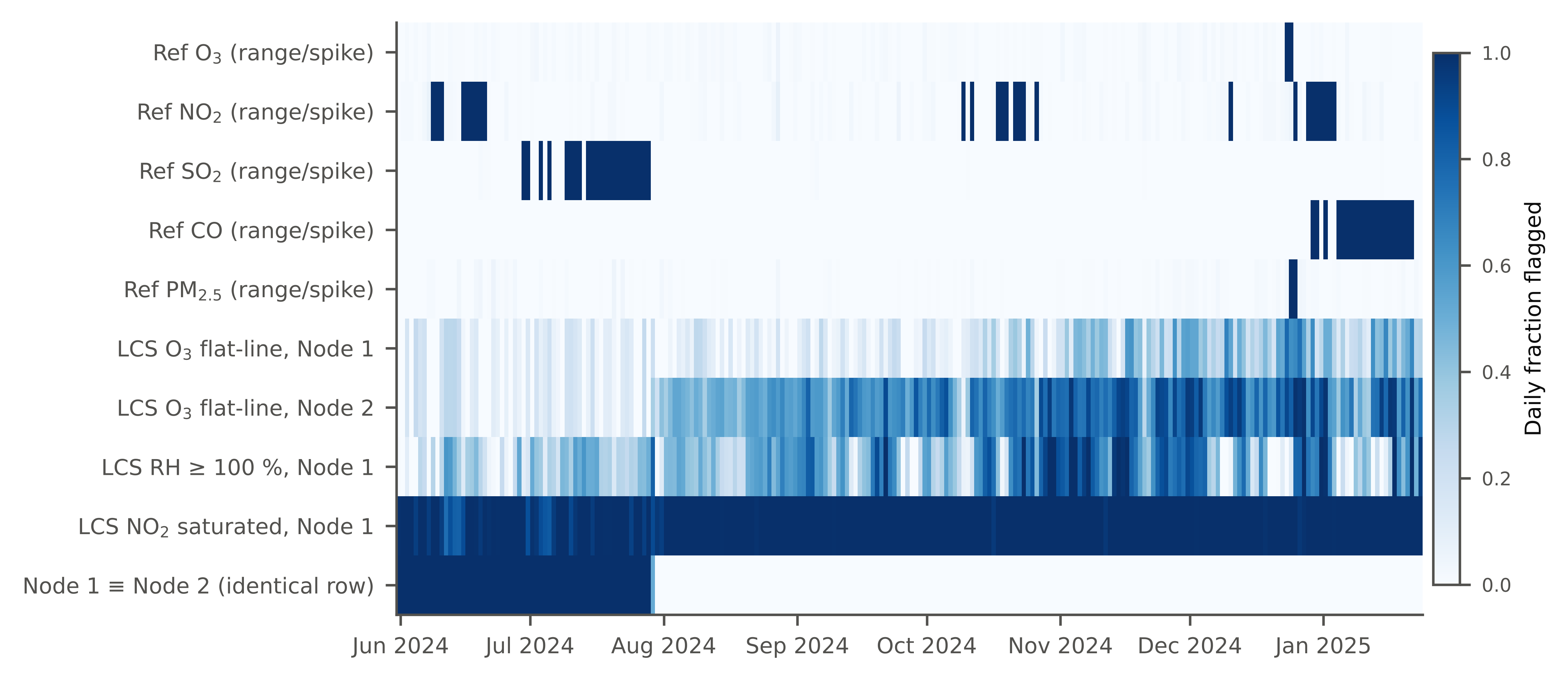
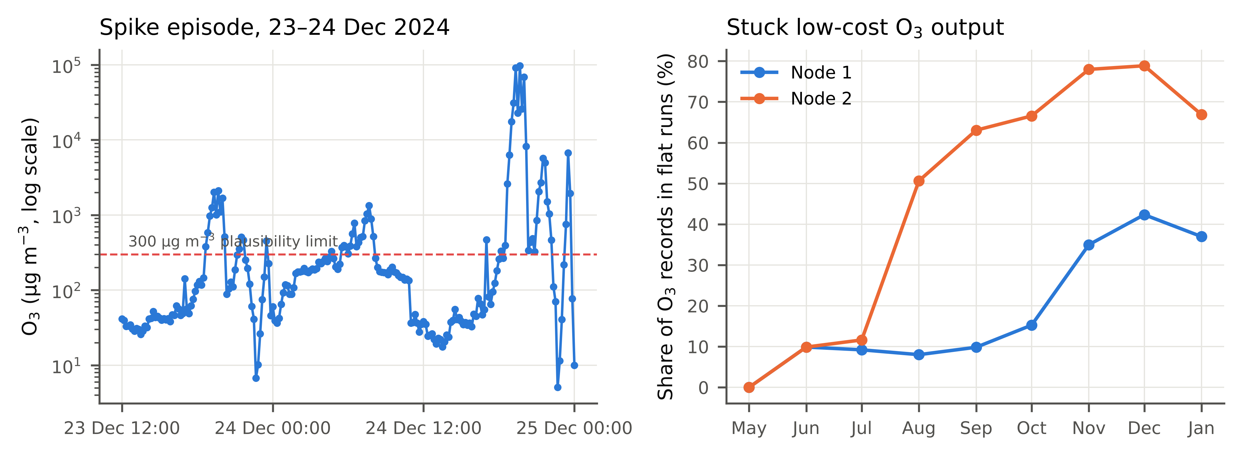
Extreme spikes. Sixty-two reference ozone values exceed 300 µg m⁻³, all on four days: 12 July, 20 November, 23 December and 24 December 2024. The largest is 97,336 µg m⁻³, at 19:40 on 24 December (Figure 2). Several of these values have a curious arithmetic structure. 97,336 is 46³, 91,125 is 45³ and 68,921 is 41³. Of the 62, 21 are exact integer squares or cubes of plausible concentrations, or simple fractions of them (for example 2,116 = 46² and 1,012.5 = 45²/2). That pattern points to a multiplicative fault somewhere in the processing chain rather than a physical event. Nitrogen oxides show the same signature at a smaller scale: NOₓ reaches −531,441, which is −81³. The other 41 values have no such structure, and between the spikes on 23–24 December the ozone record holds values of 150–250 µg m⁻³ for hours. Those values pass a 300 µg m⁻³ threshold, but they are not credible for a winter night at an urban background site. The episode rule in Eq. (2) exists to catch them.
Negative values. The reference SO₂, CO, NO, NO₂ and NOₓ series contain between 813 and 1,385 negative values each. They are not spread evenly. SO₂ negatives cluster in July 2024 (764 of 813). NO₂ negatives cluster in June 2024 (736 of 1,227). NO and NOₓ negatives cluster in June and in December–January. CO behaves strangely: every one of its 1,231 negative values is exactly −0.01 ppm, and 1,206 of them fall in January 2025, covering the whole of 17, 19 and 20 January. A constant value of −0.01 looks like a placeholder for invalid or missing data rather than a measurement.
Hidden contamination. After the range, episode and spike rules were applied, the share of reference records flagged was 1.5 % for O₃, 1.4 % for PM₂.₅, 9.7 % for SO₂, 8.9 % for CO, 8.9 % for NOₓ and 12.0 % for NO₂. Much of this is invisible in summary statistics: the reference NO₂ median is a plausible 9 µg m⁻³, even though the minimum is −13,122.
Redundant and mislabelled columns
The column documented as relative humidity (HR) in the reference files is identical to PM1 in every one of the 34,141 records, as the documentation warns. The columns PM10_S/C and PM2,5_S/C, described as readings from “a secondary or control system”, are identical to PM10 and PM2,5 in 100 % and 99.97 % of records, so they are copies rather than independent measurements. PM1_S/C is a different quantity altogether: it varies between 204.7 and 228.0 with a mean of 219.2, values that cannot be PM₁ concentrations at this site. Vac_Min is empty. The only humidity measurements in the reference files are HR_Int and Temp_Int, which describe the inside of the station enclosure, not ambient air. A user who wants ambient humidity from the reference side has nothing to use.
Health of the low-cost sensors
Several low-cost channels carry little or no information (Table 2).
-
CO is effectively constant: the most common value appears in 99.97 % of Node 1 records and 99.99 % of Node 2 records, with a standard deviation of 0.004 ppm.
-
NO₂ sits at a ceiling of 18.816 in 99.0 % of Node 1 records and 58.0 % of Node 2 records.
-
VOC is zero in 92.5–93.3 % of records.
-
RH exceeds 100 % in 46.6 % (Node 1) and 52.7 % (Node 2) of records, and is pinned at exactly 118.0 % in 8,181 Node 1 records (24 %). This looks like the sensor’s output ceiling.
-
Ozone shows the most consequential problem: stuck output. In Node 1, 20.2 % of 10-minute ozone records belong to runs of an hour or more with exactly the same value. The longest run lasts 17 hours. In Node 2 the figure is 52.6 %, and the longest run lasts more than 24 hours. Figure 2 shows that the problem grows with time. For Node 2, the share of stuck records rose from about 10 % in June to 51 % in August and 79 % in December. For Node 1 it stayed around 10 % until September, then rose to 35–42 % in November and December. PM, temperature and CO₂ never showed runs of this kind, so the stuck output is specific to the ozone channel and not a failure of the whole data logger.
| Issue | Where | Extent | Handling |
|---|---|---|---|
| Extreme spikes, some exact squares or cubes | Ref. O₃, NOₓ, NO₂, PM | 62 O₃ values > 300 µg m⁻³ on 4 days; max 97,336 | Range + episode rule |
| Negative values | Ref. SO₂, CO, NO, NO₂, NOₓ | 813–1,385 per variable, clustered by month | Range + episode rule |
| Constant negative sentinel | Ref. CO | 1,231 values of exactly −0.01 ppm, mostly January 2025 | Removed |
| Column duplicates another variable | Ref. HR = PM1 | 100 % of records | Column dropped |
| Copies presented as second system | Ref. PM10_S/C, PM2,5_S/C | 100 % / 99.97 % identical | Columns dropped |
| Unidentified quantity | Ref. PM1_S/C | Mean 219.2, range 204.7–228.0 | Column dropped |
| Hourly file inconsistent with 10-min file | All reference variables | Median Δ = 1.95 µg m⁻³ (O₃) | 10-min data aggregated by us |
| Dead or saturated channels | LCS CO, NO₂, VOC | 58–100 % of records at one value | Channels not used |
| RH above 100 %, ceiling at 118 % | LCS RH | 47–53 % of records > 100 % | Clipped at 100 % |
| Stuck ozone output | LCS O₃ | 20.2 % (Node 1), 52.6 % (Node 2) | Runs ≥ 1 h removed |
| Identical “independent” nodes | Node 1 and Node 2 | 8,524 records (25 %), until 29 July 2024 | Nodes treated as one before 30 July |
| Step change at separation | Node 2 PM₂.₅ | Mean 20.8 → 39.1 µg m⁻³ on 29–31 July | Flagged, period reported separately |
Two nodes that are one
Equation (5) gives the most surprising finding. From the first record until 29 July 2024, all eleven variables of Node 1 and Node 2 are identical at every timestamp: 8,524 records, a quarter of the dataset. Physically separate sensors never agree to full floating-point precision. Either one stream was copied into the other, or both were derived from a single device. After 29 July the streams diverge, and at that moment Node 2’s PM₂.₅ steps up abruptly: over 29–31 July its mean is 39.1 µg m⁻³, against 20.8 µg m⁻³ for Node 1.
This matters for any analysis that uses the two nodes as replicates. Inter-node agreement is the usual way to estimate the precision of a low-cost sensor model. Over the full record, the mean absolute difference between the nodes’ raw hourly ozone was 8.3 µg m⁻³. Over the period when they are actually independent, it was 11.1 µg m⁻³. For PM₂.₅ the figures were 5.4 and 7.2 µg m⁻³. Including the duplicated weeks understates the real disagreement between units by about a quarter. The correlation changed little (0.80 in both cases for ozone), so a study reporting only correlation would not notice anything.
Consequences for calibration results
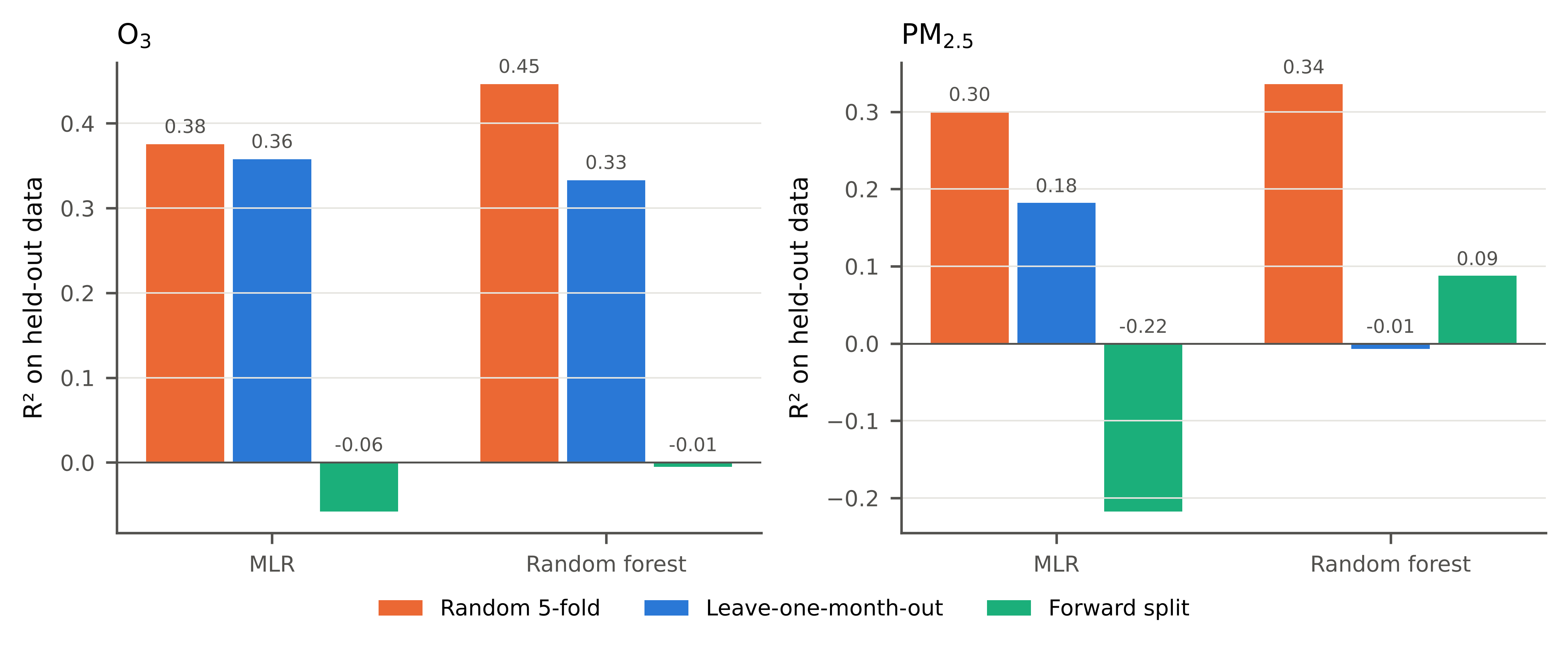
Evaluation design. The design of the test changed results more than any data problem (Table 3, Figure 3). For ozone, MLR scored R 2 = 0.38 under random folds and 0.36 under LOMO, but −0.06 on the forward split. In other words, it lost all predictive value when applied to months it had not seen bracketed by training data. The random forest showed the same pattern more strongly (0.45, 0.33 and −0.01). For PM₂.₅, MLR fell from 0.30 under random folds to 0.18 under LOMO and −0.22 forward. RF went from 0.34 to −0.01 under LOMO and 0.09 forward. By Eq. (9), random cross-validation overstated forward-looking R 2 by between 0.25 and 0.52.
| Target | Model | Rand. R² | Rand. MAE | LOMO R² | LOMO MAE | Fwd. R² | Fwd. MAE |
|---|---|---|---|---|---|---|---|
| O₃ | MLR | 0.38 | 13.15 | 0.36 | 13.41 | −0.06 | 16.68 |
| O₃ | RF | 0.45 | 12.09 | 0.33 | 13.45 | −0.01 | 16.11 |
| PM₂.₅ | MLR | 0.30 | 4.81 | 0.18 | 5.56 | −0.22 | 7.77 |
| PM₂.₅ | RF | 0.34 | 4.52 | −0.01 | 6.09 | 0.09 | 5.59 |
Replicating the published design. At 10-minute resolution, with date as an input, gradient boosting reached an MAE of 7.8 µg m⁻³ and R 2 = 0.83 on random 90/10 splits (Table 4). The same model and features, tested on the chronologically last 10 % of the record, gave an MAE of 16.0 µg m⁻³ and R 2 = −0.22. Removing the date feature from the random split raised the MAE to 12.2 µg m⁻³. The date feature therefore accounts for much of the apparent accuracy, which makes sense: with randomly interleaved test points, knowing the date lets the model interpolate between neighbouring training samples that share the same weather and the same sensor state. Under LOMO the date feature helped a little when stuck segments were kept (MAE 13.0 versus 14.1 µg m⁻³). When they were removed it made no difference to the MAE (13.9 µg m⁻³ in both cases) and slightly lowered R 2 (0.31 versus 0.33).
| Stuck runs | Features | Rand. MAE | Rand. R² | Chron. MAE | Chron. R² | LOMO MAE | LOMO R² |
|---|---|---|---|---|---|---|---|
| Kept | Date, O₃, T, RH | 7.77 | 0.83 | 16.02 | −0.22 | 13.02 | 0.53 |
| Kept | O₃, T, RH | 12.23 | 0.60 | 17.56 | −0.68 | 14.08 | 0.46 |
| Removed | Date, O₃, T, RH | 7.55 | 0.78 | 13.23 | −0.21 | 13.93 | 0.31 |
| Removed | O₃, T, RH | 12.02 | 0.48 | 15.56 | −0.79 | 13.87 | 0.33 |
Quality control. Leaving the reference spikes in place ruined the scoring entirely. With uncleaned data, LOMO RMSE for ozone was 659 µg m⁻³ for MLR and 683 µg m⁻³ for RF, and R 2 was zero or below (Table 5). A handful of values near 100,000 µg m⁻³ dominate any squared-error metric. More subtly, training on uncleaned data damaged models even when they were scored fairly against cleaned data. MLR’s MAE rose from 13.4 to 20.6 µg m⁻³ and its R 2 fell from 0.36 to −0.61. The random forest, scored the same way, produced an R 2 of −38 because a few leaves had learned to predict the corrupted spikes. PM₂.₅ was less affected, because its reference series had fewer extreme values (LOMO RMSE 12.0 µg m⁻³ uncleaned versus 9.3 µg m⁻³ cleaned for MLR).
| Data version | Model | n (h) | MAE | RMSE | R² |
|---|---|---|---|---|---|
| Quality-controlled | MLR | 4,423 | 13.41 | 17.59 | 0.36 |
| Quality-controlled | RF | 4,423 | 13.45 | 17.92 | 0.33 |
| No QC, scored on raw reference | MLR | 5,674 | 36.32 | 658.76 | 0.00 |
| No QC, scored on raw reference | RF | 5,674 | 37.40 | 682.71 | −0.08 |
| Trained without QC, scored on QC data | MLR | 4,423 | 20.62 | 27.85 | −0.61 |
| Trained without QC, scored on QC data | RF | 4,423 | 20.52 | 137.46 | −38.24 |
| QC, but stuck O₃ runs kept | MLR | 5,620 | 15.13 | 19.21 | 0.44 |
| QC, but stuck O₃ runs kept | RF | 5,620 | 13.65 | 18.41 | 0.48 |
Stuck segments. Keeping the stuck ozone segments raised R 2 even though it raised MAE (Table 5). Under LOMO, MLR went from 0.36 to 0.44 and RF from 0.33 to 0.48. With random folds, RF reached 0.58. Stuck segments are concentrated in autumn and winter, when ozone is low, so including them widens the spread of the reference values being predicted. That inflates the denominator of Eq. (8). A model can predict a low, roughly constant value for those hours and earn credit for it. Combining random folds with retained stuck segments made RF’s R 2 75 % higher than under LOMO with clean data (0.58 against 0.33), without the model having become any better at reading the sensor.
Discussion
Why these problems are easy to miss
None of the defects described here is hidden in a technical sense. Every one becomes visible with a few lines of code. They are easy to miss because they do not show up in the checks people usually run. Summary statistics of the reference NO₂ look reasonable at the median. The two nodes correlate well with each other. The 10-minute files have no missing values, which is reassuring rather than alarming at first glance. And calibration metrics computed on random folds look good. This is the pattern Sambasivan et al. (2021) described: problems that are cheap to catch at the data stage become expensive, and often invisible, once a model has been trained on them.
Some of the defects are documented and some are not. The landing page warns about outliers, negative values, the erroneous humidity column, the saturated NO₂ sensor and humidity above 100 %. It does not mention the duplicated node streams, the stuck ozone output, the copied S/C columns, the constant −0.01 CO values, the absence of gaps at 10 minutes or the inconsistency between resolutions. For several of these the data creators may have good explanations, and the original study may have handled them in ways not visible to us. The point is that a user working only from the files and the landing page cannot know.
Evaluation design dominates
The largest effect in this study came not from any data defect but from the choice of how to test. Random splitting of autocorrelated time series is a textbook form of leakage (Kapoor and Narayanan, 2023). The scale of the effect here deserves attention all the same. A model that explains 83 % of the variance under one design explains none of it under another, on the same data and with the same code. For calibration this has direct practical consequences. A calibration that looks excellent under random splitting may need recalibrating within weeks of deployment. Its users will not find this out from the published metrics.
Our reproduction of the published design differs in detail from the original study, so we do not claim that the reported MAE of about 4 µg m⁻³ would fall to any particular value under a forward test. What our results show is that the design alone can halve or double an error metric. Comparisons between calibration methods are only meaningful when the designs match, and forward-looking designs should be the default. Benchmarks of many regression algorithms against each other (Kumar and Sahu, 2021) are only as informative as the evaluation design behind them. This echoes the emphasis on site and time transferability in recent calibration work (Nowack et al., 2021; Abu-Hani et al., 2024; Hayward et al., 2025) and the push towards long-term evaluation of deployed sensors (Winter et al., 2025; Gäbel and Hertig, 2026).
Quality control is a modelling decision
Quality-control choices are often treated as housekeeping, done before the “real” analysis and described in a sentence. Our results suggest they deserve the same reporting as model hyperparameters. Removing or keeping stuck segments moved RF’s LOMO R 2 from 0.33 to 0.48, a larger change than most published comparisons between calibration algorithms. The direction was also counter-intuitive: keeping the bad data made the model look better. An author who tried both and reported the better number would not be doing anything obviously wrong, which is why the choice needs to be stated.
Our own rules involve choices too. The 300 µg m⁻³ limit, the three-violation episode rule, the Hampel parameters and the one-hour flat-run threshold are reasonable, but others could be defended. AlSalehy and Bailey (2025) showed that the treatment of outliers and missing values in multi-site gas and weather data materially affects downstream analysis, and our results point the same way. Reporting the rules and, ideally, the share of data each one removed lets readers judge for themselves. Large networks are moving towards automated, in-situ approaches to baseline correction and data screening (Mei et al., 2025), and those systems need clearly stated rules just as much as one-off studies do.
Replicates that are not replicates
The duplicated node streams deserve particular mention, because they would quietly bias several common analyses. Inter-unit precision would be overstated, as shown above. A calibration trained on one node and tested on the other would be tested partly on its own training data. A network study might count two sensors where there was effectively one. More generally, the episode is a reminder that “two devices” in a file name is a claim about provenance, and it should be verified like any other. Studies that plan co-location around repeated campaigns (Levy Zamora et al., 2023; Miech et al., 2023) depend on knowing exactly which device produced which record. The abrupt step in Node 2’s PM₂.₅ at the moment the streams separate suggests a change in hardware, firmware or data routing at that time. Without a log, the cause cannot be established.
A checklist for co-location data
Drawing these lessons together, we suggest the following minimum checks before a co-location dataset is used for calibration research, and the corresponding information that publishers should provide. They follow the spirit of datasheets for datasets (Gebru et al., 2021), adapted to sensor data.
| Topic | Users should check | Publishers should document |
|---|---|---|
| Provenance | Whether “independent” units ever produce identical values (Eq. 5) | Device identifiers, firmware changes and any period of shared or copied data |
| Timing and gaps | Gaps at every resolution; whether coarser files are averages of finer ones (Eq. 6) | How each resolution was produced; whether and how gaps were filled |
| Reference validity | Range violations, episodes and spikes (Eqs. 1–3); sentinel values | The reference network’s validity flags, or their absence |
| Sensor health | Stuck runs (Eq. 4), saturation ceilings, constant channels | Known sensor faults and maintenance events |
| Column semantics | Exact duplicates between columns; implausible units | A data dictionary with units and the instrument behind each column |
| Evaluation | Forward-looking or blocked designs; no calendar features unless justified | The design used in any accompanying paper, and its rationale |
| Reporting | Share of data removed by each QC rule; results with and without key QC choices | Recommended QC steps and their effect |
Relevance for networks in Nigeria and West Africa
The problems documented here are not unique to Valencia. If anything, they are more likely in networks built quickly, with limited reference infrastructure and limited staff time for data management, which describes most low-cost networks in sub-Saharan Africa (Awokola et al., 2022; Okure et al., 2022; Raheja et al., 2022; Raheja et al., 2023; Bittner et al., 2022). Recent reviews identify data quality and harmonisation as central challenges for these networks as they grow (Bagkis et al., 2025). Such networks will increasingly share data and build regional calibration models, and published European and North American datasets will be used to pre-train or benchmark those models. Auditing borrowed data before use, and documenting local data well enough that others can audit it, is cheap insurance. For a new Nigerian co-location campaign, the checklist in Table 6 costs a few hours of work. Discovering its lessons after a model has been deployed costs far more.
Limitations
We audited one dataset, and we cannot verify the causes of the defects we found, only their presence. Some apparent defects may have explanations not recorded in the release, such as a deliberate choice to fill gaps in the 10-minute data. The consequence experiments used two simple models and one set of features. More complex models are likely to be more sensitive to leakage, not less. Our replication of the original evaluation design was approximate. Finally, we did not have access to the reference network’s own validity flags, which would allow a cleaner separation between instrument faults and processing errors.
Conclusions
A careful look at one public co-location dataset found a dozen distinct problems, roughly half of them not mentioned in its documentation. They include corrupted reference spikes with an arithmetic signature, sentinel-like negative values, mislabelled and duplicated columns, hourly files that disagree with 10-minute files, dead and saturated sensor channels, stuck ozone output and two supposedly independent sensor nodes whose records are identical for eight weeks. Each would bias a calibration study in a predictable way. The evaluation design mattered more than any single defect. The same gradient-boosting model looked excellent under a random split with a date feature and worthless when tested on the future. Keeping stuck segments, a seemingly minor choice, raised the apparent skill of a random forest by half. Co-location data deserve the same scrutiny as the models trained on them. A short audit, a forward-looking test and transparent reporting of quality-control choices would make published calibration results much easier to trust and to compare.
Data availability
The audited dataset is openly available from Zenodo under a CC BY 4.0 licence (Montalbán Faet et al., 2025; https://doi.org/10.5281/zenodo.17044034).
Code availability
The Python scripts implementing the audit checks and the consequence experiments are available from the corresponding author on request.
Author contributions
R. E. Ogu: Conceptualization, Methodology, Software, Validation, Writing – original draft, review and editing.
Competing interests
The authors declare no competing interests.
Acknowledgements
The author is grateful to the creators of the Molí del Sol dataset for releasing their data openly. Without open data, an audit of this kind would not be possible, and this paper should be read as support for that practice.
References
- Abu-Hani, A., Chen, J., Balamurugan, V., Wenzel, A., & Bigi, A. (2024). Transferability of machine-learning-based global calibration models for NO2 and NO low-cost sensors. Atmospheric Measurement Techniques, 17(13), 3917–3931. DOI ↗ Google Scholar ↗
- AlSalehy, A. S., & Bailey, M. (2025). Improving time series data quality: Identifying outliers and handling missing values in a multilocation gas and weather dataset. Smart Cities, 8(3), 82. DOI ↗ Google Scholar ↗
- Awokola, B., Okello, G., Johnson, O., Dobson, R., Ouédraogo, A. R., Dibba, B., et al. (2022). Longitudinal ambient PM2.5 measurement at fifteen locations in eight sub-Saharan African countries using low-cost sensors. Atmosphere, 13(10), 1593. DOI ↗ Google Scholar ↗
- Bagkis, E., Hassani, A., Schneider, P., DeSouza, P., Shetty, S., Kassandros, T., et al. (2025). Evolving trends in application of low-cost air quality sensor networks: Challenges and future directions. npj Climate and Atmospheric Science, 8, 335. DOI ↗ Google Scholar ↗
- Bagkis, E., Kassandros, T., & Karatzas, K. (2022). Learning calibration functions on the fly: Hybrid batch online stacking ensembles for the calibration of low-cost air quality sensor networks in the presence of concept drift. Atmosphere, 13(3), 416. DOI ↗ Google Scholar ↗
- Bittner, A. S., Cross, E. S., Hagan, D. H., Malings, C., Lipsky, E., & Grieshop, A. P. (2022). Performance characterization of low-cost air quality sensors for off-grid deployment in rural Malawi. Atmospheric Measurement Techniques, 15(11), 3353–3376. DOI ↗ Google Scholar ↗
- Concas, F., Mineraud, J., Lagerspetz, E., Varjonen, S., Liu, X., Puolamäki, K., Nurmi, P., & Tarkoma, S. (2021). Low-cost outdoor air quality monitoring and sensor calibration: A survey and critical analysis. ACM Transactions on Sensor Networks, 17(2), 1–44. DOI ↗ Google Scholar ↗
- deSouza, P., Barkjohn, K., Clements, A., Lee, J., Kahn, R., Crawford, B., & Kinney, P. (2023). An analysis of degradation in low-cost particulate matter sensors. Environmental Science: Atmospheres, 3(3), 521–536. DOI ↗ Google Scholar ↗
- deSouza, P., Kahn, R., Stockman, T., Obermann, W., Crawford, B., Wang, A., et al. (2022). Calibrating networks of low-cost air quality sensors. Atmospheric Measurement Techniques, 15(21), 6309–6328. DOI ↗ Google Scholar ↗
- Diez, S., Lacy, S. E., Bannan, T. J., Flynn, M., Gardiner, T., Harrison, D., et al. (2022). Air pollution measurement errors: Is your data fit for purpose?. Atmospheric Measurement Techniques, 15(13), 4091–4105. DOI ↗ Google Scholar ↗
- Gäbel, P., & Hertig, E. (2026). Recalibration of low-cost O3 and PM2.5 sensors: Linking practices to recent air sensor test protocols. Atmospheric Measurement Techniques, 19, 1293–1321. DOI ↗ Google Scholar ↗
- Gama, J., Žliobaitė, I., Bifet, A., Pechenizkiy, M., & Bouchachia, A. (2014). A survey on concept drift adaptation. ACM Computing Surveys, 46(4), 1–37. DOI ↗ Google Scholar ↗
- Gebru, T., Morgenstern, J., Vecchione, B., Vaughan, J. W., Wallach, H., Daumé III, H., & Crawford, K. (2021). Datasheets for datasets. Communications of the ACM, 64(12), 86–92. DOI ↗ Google Scholar ↗
- Giordano, M. R., Malings, C., Pandis, S. N., Presto, A. A., McNeill, V. F., Westervelt, D. M., et al. (2021). From low-cost sensors to high-quality data: A summary of challenges and best practices for effectively calibrating low-cost particulate matter mass sensors. Journal of Aerosol Science, 158, 105833. DOI ↗ Google Scholar ↗
- Hayward, I., Martin, N. A., Ferracci, V., Kazemimanesh, M., Jude, S., Walton, C., et al. (2025). Comprehensive comparison of correction techniques for low-cost air quality sensors: The impact of device type and deployment environment. npj Climate and Atmospheric Science, 8, 389. DOI ↗ Google Scholar ↗
- Kang, Y., Aye, L., Ngo, T. D., & Zhou, J. (2022). Performance evaluation of low-cost air quality sensors: A review. Science of the Total Environment, 818, 151769. DOI ↗ Google Scholar ↗
- Kapoor, S., & Narayanan, A. (2023). Leakage and the reproducibility crisis in machine-learning-based science. Patterns, 4(9), 100804. DOI ↗ Google Scholar ↗
- Kumar, V., & Sahu, M. (2021). Evaluation of nine machine learning regression algorithms for calibration of low-cost PM2.5 sensor. Journal of Aerosol Science, 157, 105809. DOI ↗ Google Scholar ↗
- Levy Zamora, M., Buehler, C., Datta, A., Gentner, D. R., & Koehler, K. (2023). Identifying optimal co-location calibration periods for low-cost sensors. Atmospheric Measurement Techniques, 16(1), 169–179. DOI ↗ Google Scholar ↗
- Li, J., Hauryliuk, A., Malings, C., Eilenberg, S. R., Subramanian, R., & Presto, A. A. (2021). Characterizing the aging of Alphasense NO2 sensors in long-term field deployments. ACS Sensors, 6(8), 2952–2959. DOI ↗ Google Scholar ↗
- Liang, L. (2021). Calibrating low-cost sensors for ambient air monitoring: Techniques, trends, and challenges. Environmental Research, 197, 111163. DOI ↗ Google Scholar ↗
- Malings, C., Tanzer, R., Hauryliuk, A., Kumar, S. P. N., Zimmerman, N., Kara, L. B., Presto, A. A., & Subramanian, R. (2019). Development of a general calibration model and long-term performance evaluation of low-cost sensors for air pollutant gas monitoring. Atmospheric Measurement Techniques, 12(2), 903–920. DOI ↗ Google Scholar ↗
- Mei, H., Wei, P., Wang, Y., Ghadikolaei, M. A., Gali, N. K., & Ning, Z. (2025). In-situ baseline calibration approach for enhanced data quality of large-scale air sensor monitoring networks. npj Climate and Atmospheric Science, 8, 296. DOI ↗ Google Scholar ↗
- Miech, J. A., Stanton, L., Gao, M., Micalizzi, P., Uebelherr, J., Herckes, P., & Fraser, M. P. (2023). In situ drift correction for a low-cost NO2 sensor network. Environmental Science: Atmospheres, 3(5), 894–904. DOI ↗ Google Scholar ↗
- Montalbán Faet, G., Meneses Albalá, E., Felici-Castell, S., Pérez Solano, J. J., & Segura-Garcia, J. (2025). Air quality data from regulatory AQMS and low-cost sensors in Molí del Sol, Valencia (May 31 2024 – January 23, 2025) (Version 1.0.0) [Data set]. Zenodo. DOI ↗ Google Scholar ↗
- Montalbán-Faet, G., Meneses-Albalá, E., Felici-Castell, S., Pérez-Solano, J. J., & Segura-Garcia, J. (2025). Improving raw readings from low-cost ozone sensors using artificial intelligence for air quality monitoring. Atmospheric Measurement Techniques, 18, 4357–4372. DOI ↗ Google Scholar ↗
- Nowack, P., Konstantinovskiy, L., Gardiner, H., & Cant, J. (2021). Machine learning calibration of low-cost NO2 and PM10 sensors: Non-linear algorithms and their impact on site transferability. Atmospheric Measurement Techniques, 14(8), 5637–5655. DOI ↗ Google Scholar ↗
- Okorn, K., & Iraci, L. T. (2024). An overview of outdoor low-cost gas-phase air quality sensor deployments: Current efforts, trends, and limitations. Atmospheric Measurement Techniques, 17(21), 6425–6457. DOI ↗ Google Scholar ↗
- Okure, D., Ssematimba, J., Sserunjogi, R., Gracia, N. L., Soppelsa, M. E., & Bainomugisha, E. (2022). Characterization of ambient air quality in selected urban areas in Uganda using low-cost sensing and measurement technologies. Environmental Science & Technology, 56(6), 3324–3339. DOI ↗ Google Scholar ↗
- Raheja, G., Nimo, J., Appoh, E. K.-E., Essien, B., Sunu, M., Nyante, J., et al. (2023). Low-cost sensor performance intercomparison, correction factor development, and 2+ years of ambient PM2.5 monitoring in Accra, Ghana. Environmental Science & Technology, 57(29), 10708–10720. DOI ↗ Google Scholar ↗
- Raheja, G., Sabi, K., Sonla, H., Gbedjangni, E. K., McFarlane, C. M., Hodoli, C. G., & Westervelt, D. M. (2022). A network of field-calibrated low-cost sensor measurements of PM2.5 in Lomé, Togo, over one to two years. ACS Earth and Space Chemistry, 6(4), 1011–1021. DOI ↗ Google Scholar ↗
- Sambasivan, N., Kapania, S., Highfill, H., Akrong, D., Paritosh, P., & Aroyo, L. M. (2021). “Everyone wants to do the model work, not the data work”: Data cascades in high-stakes AI. Proceedings of the 2021 CHI Conference on Human Factors in Computing Systems, 1–15. DOI ↗ Google Scholar ↗
- Schmitz, S., Towers, S., Villena, G., Caseiro, A., Wegener, R., Klemp, D., et al. (2021). Unravelling a black box: An open-source methodology for the field calibration of small air quality sensors. Atmospheric Measurement Techniques, 14(11), 7221–7241. DOI ↗ Google Scholar ↗
- Van Poppel, M., Schneider, P., Peters, J., Yatkin, S., Gerboles, M., Matheeussen, C., et al. (2023). SensEURCity: A multi-city air quality dataset collected for 2020/2021 using open low-cost sensor systems. Scientific Data, 10, 322. DOI ↗ Google Scholar ↗
- Whang, S. E., Roh, Y., Song, H., & Lee, J.-G. (2023). Data collection and quality challenges in deep learning: A data-centric AI perspective. The VLDB Journal, 32(4), 791–813. DOI ↗ Google Scholar ↗
- Winter, A. R., Zhu, Y., Asimow, N. G., Patel, M. Y., & Cohen, R. C. (2025). Sustained performance of low-cost air quality sensors in long-term deployments. ACS Sensors, 10(6), 4329–4335. DOI ↗ Google Scholar ↗
- Zimmerman, N., Presto, A. A., Kumar, S. P. N., Gu, J., Hauryliuk, A., Robinson, E. S., Robinson, A. L., & Subramanian, R. (2018). A machine learning calibration model using random forests to improve sensor performance for lower-cost air quality monitoring. Atmospheric Measurement Techniques, 11(1), 291–313. DOI ↗ Google Scholar ↗